---
title: 重采样方法的数据分割
---
flowchart TD
A(原始数据) --> B[[训练集]]
A --> C[[测试集]]
B --> D{{重采样1}}
B --> E{{重采样2}}
B --> F{{重采样n}}
D --> G[[分析集]]
D --> H[[评估集]]
E --> I[[分析集]]
E --> J[[评估集]]
F --> K[[分析集]]
F --> L[[评估集]]
D -.- E
E -.- F
3 tidymodels-进阶
3.1 重采样方法
偏倚bias:数据中的真实模式或关系与模型所能模拟的模式类型之间的差异。运用合理的重采样方法,可以有效减小偏倚。
重采样只在训练集上进行,测试集不参与重采样。每次重采样,训练集都会被划分为分析集和评估集。分析集用于训练模型,评估集用于评估模型的性能,如 图 3.1 所示。模型性能的最终估计值是所有评估集重复统计的平均值。
3.1.1 交叉验证CV
k折交叉验证k-CV
交叉验证是一种重采样方法,最常见的是k折交叉验证。在k折交叉验证中,数据被分为k个子集,其中一个子集被保留作为评估集,其余k-1个子集被用于训练模型。这个过程重复k次,每个子集都有一次机会作为评估集。最后,模型性能的最终估计值是所有评估集重复统计的平均值。
vfold_cv()函数可以用于创建k折交叉验证。
重要
k值越大,重取样估计值偏倚越小,但方差越大。通常k值取5或10。
代码
set.seed(123)
tidymodels_prefer()

# 10折交叉验证
ames_train |>
  vfold_cv(v = 10) -> ames_folds
ames_folds
# 10-fold cross-validation
# A tibble: 10 × 2
splits id
<list> <chr>
1 <split [2107/235]> Fold01
2 <split [2107/235]> Fold02
3 <split [2108/234]> Fold03
4 <split [2108/234]> Fold04
5 <split [2108/234]> Fold05
6 <split [2108/234]> Fold06
7 <split [2108/234]> Fold07
8 <split [2108/234]> Fold08
9 <split [2108/234]> Fold09
10 <split [2108/234]> Fold10重复k折交叉验证repeated k-CV
重复k折交叉验证是k折交叉验证的扩展,它重复k折交叉验证多次。重复k折交叉验证的优点是它提供了更准确的模型性能估计,但是计算成本更高。
在vfold_cv()函数中,可以使用repeats参数指定重复次数。
代码
ames_train |>
  vfold_cv(v = 10, repeats = 5)
# 10-fold cross-validation repeated 5 times
# A tibble: 50 × 3
splits id id2
<list> <chr> <chr>
1 <split [2107/235]> Repeat1 Fold01
2 <split [2107/235]> Repeat1 Fold02
3 <split [2108/234]> Repeat1 Fold03
4 <split [2108/234]> Repeat1 Fold04
5 <split [2108/234]> Repeat1 Fold05
6 <split [2108/234]> Repeat1 Fold06
7 <split [2108/234]> Repeat1 Fold07
8 <split [2108/234]> Repeat1 Fold08
9 <split [2108/234]> Repeat1 Fold09
10 <split [2108/234]> Repeat1 Fold10
# ℹ 40 more rows留一法LOO
留一法LOO是k折交叉验证的一个特例,其中k等于训练集的观测数。这时,每个评估集只包含一个观测。LOO的优点是它提供了最小的偏倚,但是计算成本很高。一般来说,LOO不适用于大型数据集。
蒙特卡罗交叉验证MCCV
蒙特卡罗交叉验证是一种重复随机划分数据的方法。在每次重复中,数据被随机划分为训练集和评估集,且最终产生的评估集互斥。这种方法的优点是它可以提供更准确的模型性能估计,但是计算成本更高。
mc_cv()函数可以用于创建蒙特卡罗交叉验证。其中,prop参数指定训练集的比例,times参数指定重复次数。
代码
ames_train |>
  mc_cv(prop = 9/10, times = 20)
# Monte Carlo cross-validation (0.9/0.1) with 20 resamples
# A tibble: 20 × 2
splits id
<list> <chr>
1 <split [2107/235]> Resample01
2 <split [2107/235]> Resample02
3 <split [2107/235]> Resample03
4 <split [2107/235]> Resample04
5 <split [2107/235]> Resample05
6 <split [2107/235]> Resample06
7 <split [2107/235]> Resample07
8 <split [2107/235]> Resample08
9 <split [2107/235]> Resample09
10 <split [2107/235]> Resample10
11 <split [2107/235]> Resample11
12 <split [2107/235]> Resample12
13 <split [2107/235]> Resample13
14 <split [2107/235]> Resample14
15 <split [2107/235]> Resample15
16 <split [2107/235]> Resample16
17 <split [2107/235]> Resample17
18 <split [2107/235]> Resample18
19 <split [2107/235]> Resample19
20 <split [2107/235]> Resample203.1.2 验证集
验证集方法其实是只进行一次重采样,将数据分为训练集和验证集。验证集方法的优点是计算成本低,但是它提供的模型性能估计可能不准确。
代码
ames |>
  initial_validation_split(prop = c(0.6, 0.2)) |> # 训练集60%,验证集20%,测试集20%
  validation_set() # 验证集
# A tibble: 1 × 2
splits id
<list> <chr>
1 <split [1758/586]> validation3.1.3 Bootstrap
Bootstrap是一种重采样方法,它通过有放回地抽样来创建新的数据集。在每次重采样中,数据集的大小保持不变,但是每个观测可以被多次抽样。Bootstrap的优点是产生的性能估计方差较小,但是它可能产生较大的偏倚,尤其会低估准确率。
bootstraps()函数可以用于创建Bootstrap。
代码
ames_train |>
  bootstraps(times = 10)
# Bootstrap sampling
# A tibble: 10 × 2
splits id
<list> <chr>
1 <split [2342/881]> Bootstrap01
2 <split [2342/868]> Bootstrap02
3 <split [2342/896]> Bootstrap03
4 <split [2342/852]> Bootstrap04
5 <split [2342/861]> Bootstrap05
6 <split [2342/871]> Bootstrap06
7 <split [2342/852]> Bootstrap07
8 <split [2342/857]> Bootstrap08
9 <split [2342/857]> Bootstrap09
10 <split [2342/880]> Bootstrap103.1.4 滚动抽样-时间序列
滚动预测原点重采样方法是一种时间序列数据的重采样方法。初始训练集和评估集的大小是指定的。重采样的第一次迭代从序列的起点开始。第二次迭代向后移位一定数量的样本。流程如 图 3.2 所示。

假设有一个时间序列数据集,由6组30天的数据块组成。可以设置初始训练集和评估集的大小为30天。第一次迭代,训练集包含第1-30天的数据,评估集包含第31-60天的数据。第二次迭代,训练集包含第31-60天的数据,评估集包含第61-90天的数据。以此类推。
rolling_origin()函数可以用于创建滚动预测原点重采样。
代码
tibble(x = 1:365) |>
  rolling_origin(initial = 6 * 30, # 初始训练集大小
                 assess = 30, # 评估集大小
                 skip = 29, # 每次迭代的跳跃步长
                 cumulative = FALSE) -> time_slices # 是否累积

data_range <- function(x) {
  summarise(x, first = min(x), last = max(x))
}

time_slices$splits |>
  map_dfr(~ analysis(.x) |>
            data_range())
# A tibble: 6 × 2
first last
<int> <int>
1 1 180
2 31 210
3 61 240
4 91 270
5 121 300
6 151 330代码
time_slices$splits |>
  map_dfr(~ assessment(.x) |>
            data_range())
# A tibble: 6 × 2
first last
<int> <int>
1 181 210
2 211 240
3 241 270
4 271 300
5 301 330
6 331 3603.2 评估重采样性能
首先建立一个随机森林模型。
代码
rf_model <-
  rand_forest(trees = 1000) |>
  set_engine("ranger") |>
  set_mode("regression")

rf_workflow <-
  workflow() |>
  add_formula(
    Sale_Price ~ Neighborhood + Gr_Liv_Area +
      Year_Built + Bldg_Type + Latitude + Longitude
  ) |>
  add_model(rf_model)

rf_fit <-
  rf_workflow |>
  fit(data = ames_train)
3.2.1 十折交叉验证
使用control_resamples()函数设置模型重采样控制参数;使用fit_resamples()函数对模型进行重采样训练和评估。
代码
keep_pred <-
  control_resamples(save_pred = TRUE, save_workflow = TRUE)

ames_train |>
  vfold_cv(v = 10) -> ames_folds

set.seed(123)
rf_workflow |>
  fit_resamples(
    resamples = ames_folds,
    control = keep_pred
  ) -> rf_res

rf_res
# Resampling results
# 10-fold cross-validation
# A tibble: 10 × 5
splits id .metrics .notes .predictions
<list> <chr> <list> <list> <list>
1 <split [2107/235]> Fold01 <tibble [2 × 4]> <tibble [0 × 3]> <tibble>
2 <split [2107/235]> Fold02 <tibble [2 × 4]> <tibble [0 × 3]> <tibble>
3 <split [2108/234]> Fold03 <tibble [2 × 4]> <tibble [0 × 3]> <tibble>
4 <split [2108/234]> Fold04 <tibble [2 × 4]> <tibble [0 × 3]> <tibble>
5 <split [2108/234]> Fold05 <tibble [2 × 4]> <tibble [0 × 3]> <tibble>
6 <split [2108/234]> Fold06 <tibble [2 × 4]> <tibble [0 × 3]> <tibble>
7 <split [2108/234]> Fold07 <tibble [2 × 4]> <tibble [0 × 3]> <tibble>
8 <split [2108/234]> Fold08 <tibble [2 × 4]> <tibble [0 × 3]> <tibble>
9 <split [2108/234]> Fold09 <tibble [2 × 4]> <tibble [0 × 3]> <tibble>
10 <split [2108/234]> Fold10 <tibble [2 × 4]> <tibble [0 × 3]> <tibble> 在rf_res中,包含了每次重采样的模型性能评估结果。可以使用collect_metrics()函数提取模型性能指标。
代码
rf_res |>
  collect_metrics()
# A tibble: 2 × 6
.metric .estimator mean n std_err .config
<chr> <chr> <dbl> <int> <dbl> <chr>
1 rmse standard 0.0728 10 0.00261 Preprocessor1_Model1
2 rsq standard 0.830 10 0.0111 Preprocessor1_Model1方法的模型性能评估结果可以使用collect_predictions()函数提取。
代码
rf_res |>
  collect_predictions() -> assess_res

assess_res
# A tibble: 2,342 × 5
.pred id .row Sale_Price .config
<dbl> <chr> <int> <dbl> <chr>
1 5.07 Fold01 1 5.10 Preprocessor1_Model1
2 5.17 Fold01 16 5.04 Preprocessor1_Model1
3 4.91 Fold01 27 4.90 Preprocessor1_Model1
4 5.04 Fold01 37 5.09 Preprocessor1_Model1
5 5.02 Fold01 40 5.04 Preprocessor1_Model1
6 5.15 Fold01 44 4.97 Preprocessor1_Model1
7 5.12 Fold01 57 5.10 Preprocessor1_Model1
8 4.98 Fold01 60 4.90 Preprocessor1_Model1
9 4.92 Fold01 69 5.01 Preprocessor1_Model1
10 5.08 Fold01 78 4.88 Preprocessor1_Model1
# ℹ 2,332 more rows对性能评估结果assess_res进行可视化,如 图 3.3 所示。
代码
assess_res |>
  ggplot(aes(x = Sale_Price, y = .pred)) +
  geom_point(alpha = 0.15) +
  # 把x<4.5的点标记成红色
  geom_point(data = filter(assess_res, Sale_Price < 4.5), color = "red", alpha = 0.25) +
  geom_abline(color = "red") +
  coord_obs_pred() +
  theme_bw() +
  ylab("Predicted")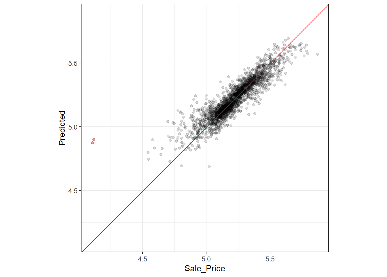
图 3.3 中,标红的两个点表示销售价格较低的这两个房屋预测值大大偏高。可以在assess_res中定位到这两个数据,进而分析特定预测性能较差的可能原因。
代码
over_predicted <-
  assess_res |>
  mutate(residual = Sale_Price - .pred) |> # 计算残差
  arrange(desc(abs(residual))) |> # 按残差绝对值降序排列
  slice(1:2) # 取前两个数据

over_predicted
# A tibble: 2 × 6
.pred id .row Sale_Price .config residual
<dbl> <chr> <int> <dbl> <chr> <dbl>
1 4.90 Fold03 319 4.12 Preprocessor1_Model1 -0.783
2 4.87 Fold06 32 4.11 Preprocessor1_Model1 -0.767代码
ames_train |>
  slice(over_predicted$.row) |> # 取出这两个数据
  select(Gr_Liv_Area, Neighborhood, Year_Built, Bedroom_AbvGr, Full_Bath) # 选择感兴趣的变量
# A tibble: 2 × 5
Gr_Liv_Area Neighborhood Year_Built Bedroom_AbvGr Full_Bath
<int> <fct> <int> <int> <int>
1 733 Iowa_DOT_and_Rail_Road 1952 2 1
2 832 Old_Town 1923 2 13.2.2 验证集
使用fit_resamples()函数对模型进行重采样训练和评估。
代码
ames |>
  initial_validation_split(prop = c(0.6, 0.2)) |>
  validation_set() -> val_set # 划分验证集

rf_workflow |>
  fit_resamples(resamples = val_set) -> val_res # 对验证集进行重采样训练和评估

val_res
# Resampling results
# Validation Set (0.75/0.25)
# A tibble: 1 × 4
splits id .metrics .notes
<list> <chr> <list> <list>
1 <split [1758/586]> validation <tibble [2 × 4]> <tibble [0 × 3]>代码
collect_metrics(val_res) # 提取模型性能指标# A tibble: 2 × 6
.metric .estimator mean n std_err .config
<chr> <chr> <dbl> <int> <dbl> <chr>
1 rmse standard 0.0657 1 NA Preprocessor1_Model1
2 rsq standard 0.845 1 NA Preprocessor1_Model13.3 并行计算
tune包使用foreach包来进行并行计算。
parallel包可以计算本机的并行计算能力。
代码
parallel::detectCores(logical = FALSE) # 物理核心数[1] 12代码
parallel::detectCores(logical = TRUE) # 逻辑核心数,包括超线程[1] 16doParallel包可以使用registerDoParallel()函数注册并行计算。
代码
library(doParallel)

cl <- makePSOCKcluster(4) # 创建4个核心的并行计算集群
registerDoParallel(cl) # 注册并行计算

## 运行fit_resamples()函数----------------

stopCluster(cl) # 关闭并行计算集群
3.4 利用重采样方法比较模型
代码
rm(list = ls())
load("../data/tidymodels_2_1.rda")
3.4.1 建立多个模型
建立三个不同的线性回归模型。
代码
## 基本模型----------------
basic_rec <-
  ames_train |>
  recipe(Sale_Price ~ Neighborhood + Gr_Liv_Area + Year_Built + Bldg_Type +
           Latitude + Longitude) |>
  step_log(Gr_Liv_Area, base = 10) |>
  step_other(Neighborhood, threshold = 0.01) |>
  step_dummy(all_nominal_predictors())

## 基本模型 + 交互项----------------
interaction_rec <-
  basic_rec |>
  step_interact( ~ Gr_Liv_Area:starts_with("Bldg_Type_"))

## 基本模型 + 交互项 + 自然样条----------------
spline_rec <-
  interaction_rec |>
  step_ns(Latitude, Longitude, deg_free = 50)

## 建立模型----------------
preproc <-
  list(basic = basic_rec,
       interact = interaction_rec,
       splines = spline_rec
  )

lm_models <-
  preproc |>
  workflow_set(list(lm = linear_reg()), cross = FALSE) # 建立线性回归模型,不进行重采样

lm_models
# A workflow set/tibble: 3 × 4
wflow_id info option result
<chr> <list> <list> <list>
1 basic_lm <tibble [1 × 4]> <opts[0]> <list [0]>
2 interact_lm <tibble [1 × 4]> <opts[0]> <list [0]>
3 splines_lm <tibble [1 × 4]> <opts[0]> <list [0]>使用workflow_map()函数对三个模型进行重采样。verbose = TRUE参数可以显示进度条,seed = 123参数可以设置随机种子。
代码
lm_models <-
  lm_models |>
  workflow_map(
    "fit_resamples",
    seed = 123,
    verbose = TRUE,
    resamples = ames_folds,
    control = keep_pred
  )

lm_models
# A workflow set/tibble: 3 × 4
wflow_id info option result
<chr> <list> <list> <list>
1 basic_lm <tibble [1 × 4]> <opts[2]> <rsmp[+]>
2 interact_lm <tibble [1 × 4]> <opts[2]> <rsmp[+]>
3 splines_lm <tibble [1 × 4]> <opts[2]> <rsmp[+]>使用collect_metrics()函数提取模型性能指标。
代码
lm_models |>
  collect_metrics() |>
  filter(.metric == "rmse")
# A tibble: 3 × 9
wflow_id .config preproc model .metric .estimator mean n std_err
<chr> <chr> <chr> <chr> <chr> <chr> <dbl> <int> <dbl>
1 basic_lm Preprocesso… recipe line… rmse standard 0.0794 10 0.00318
2 interact_lm Preprocesso… recipe line… rmse standard 0.0789 10 0.00320
3 splines_lm Preprocesso… recipe line… rmse standard 0.0777 10 0.00308添加其他模型时,需要提前在其他模型重采样流程中设置save_workflow = TRUE。使用as_workflow_set()函数将保存的工作流转换为workflow_set对象。
代码
four_models <-
  as_workflow_set(random_forest = rf_res) |>
  bind_rows(lm_models)

four_models
# A workflow set/tibble: 4 × 4
wflow_id info option result
<chr> <list> <list> <list>
1 random_forest <tibble [1 × 4]> <opts[0]> <rsmp[+]>
2 basic_lm <tibble [1 × 4]> <opts[2]> <rsmp[+]>
3 interact_lm <tibble [1 × 4]> <opts[2]> <rsmp[+]>
4 splines_lm <tibble [1 × 4]> <opts[2]> <rsmp[+]>使用autoplot()函数对模型进行可视化。
代码
library(ggrepel)
four_models |>
  autoplot(metric = "rsq") + # 可视化R^2
  geom_text_repel(aes(label = wflow_id), nudge_x = 1/8, nudge_y = 1/100) + # 添加模型名称
  theme(legend.position = "none") # 隐藏图例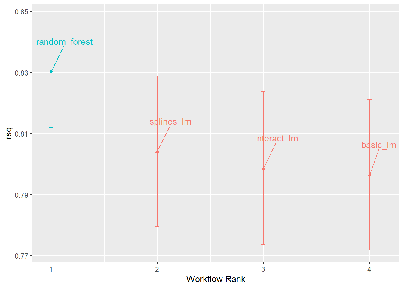
由 图 3.4 可以看出,随机森林模型的R2值最高,且随着模型复杂度的增加,R2值也在增加,说明线性模型有细微的改进。
3.4.2 比较重采样的性能统计
在不同的线性模型之间,R2值的差异并不大。但是,这种差异是否具有统计学意义仍需进一步检验。
3.4.2.1 假设检验
可以用配对t检验方法检验不同模型之间的R2值差异是否具有统计学意义。
代码
rsq_indiv_estimates <-
  four_models |>
  collect_metrics(summarize = FALSE) |> # 提取模型性能指标
  filter(.metric == "rsq") # 提取R^2^值

rsq_wider <-
  rsq_indiv_estimates |>
  select(wflow_id, .estimate, id) |>
  pivot_wider(id_cols = "id", names_from = "wflow_id", values_from = ".estimate")

corrr::correlate(rsq_wider %>% select(-id), quiet = TRUE) # 计算R^2^值的相关系数
# A tibble: 4 × 5
term random_forest basic_lm interact_lm splines_lm
<chr> <dbl> <dbl> <dbl> <dbl>
1 random_forest NA 0.925 0.933 0.915
2 basic_lm 0.925 NA 0.996 0.977
3 interact_lm 0.933 0.996 NA 0.977
4 splines_lm 0.915 0.977 0.977 NA 代码
# 基本模型和交互模型-------------------------------------------------------
rsq_wider |>
  with(t.test(splines_lm, basic_lm, paired = TRUE)) |>
  tidy() |>
  select(estimate, p.value, starts_with("conf")) # 提取估计值、p值和置信区间
# A tibble: 1 × 4
estimate p.value conf.low conf.high
<dbl> <dbl> <dbl> <dbl>
1 0.00770 0.0391 0.000480 0.0149根据假设检验结果,p值不显著,且R2值差异仅为0.77%。因此,不同模型之间的R2值差异不具有统计学意义。
3.4.2.2 贝叶斯
3.4.2.2.1 随机截距模型
使用tidyposterior包中的perf_mod()函数可以建立贝叶斯模型,并将其与重采样统计量拟合。
代码
packages <- c("tidyposterior", "rstanarm")
for (pkg in packages) {
  if (!require(pkg, character.only = TRUE, quietly = TRUE)) {
    install.packages(pkg, dependencies = TRUE)
    require(pkg, character.only = TRUE, quietly = TRUE)
  }
}

# 建立贝叶斯先验模型--------------------------------------------------------
rsq_anova <-
  four_models |>
  perf_mod(
    metric = "rsq",
    prior_intercept = rstanarm::student_t(df = 1), # 指定拟合模型时用于截距项的先验分布
    chains = 4,
    iter = 5000,
    seed = 123,
    refresh = 0 # 不显示进度条
  )

# 提取模型后验信息-----------------------------------------------------------
model_post <-
  rsq_anova |>
  tidy(seed = 1103)
代码
model_post |>
  mutate(model = forcats::fct_inorder(model)) |> # 对模型名称进行排序
  ggplot(aes(x = posterior)) +
  geom_histogram(bins = 50, color = "white", fill = "blue", alpha = 0.4) +
  facet_wrap(~ model, ncol = 1) +
  theme_bw()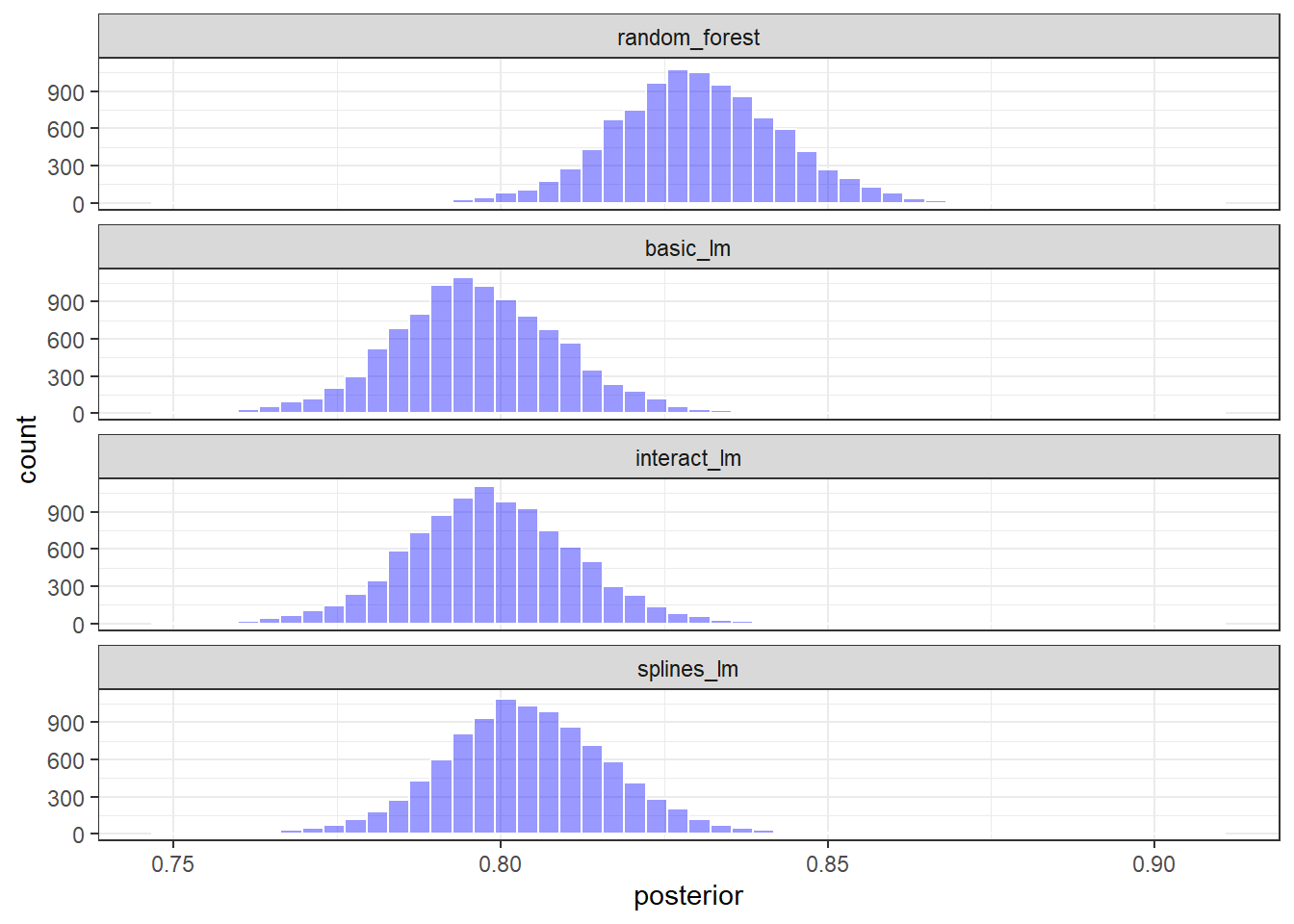
图 3.5 和 图 3.6 分别展示了不同模型的平均R2值的估计概率分布和置信区间。可以看出,各个模型的后验分布有所重叠,尤其是三个线性模型之间,说明不同模型之间的R2值差异不具有统计学意义。
代码
rsq_anova |>
  autoplot() +
  geom_text_repel(aes(label = workflow), nudge_x = 1/8, nudge_y = 1/100) +
  theme(legend.position = "none")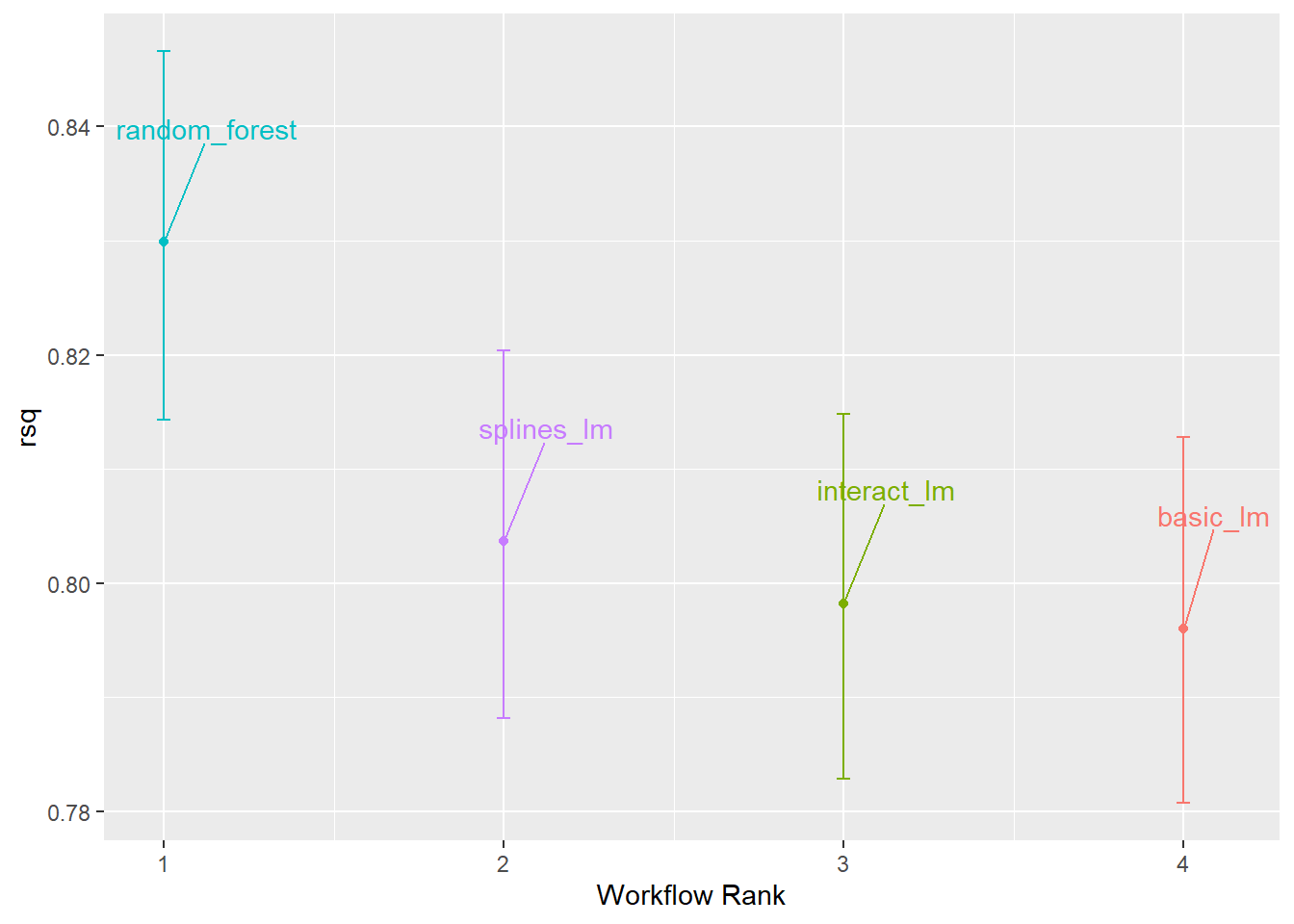
使用contrast_models()函数对不同模型的R2差异的后验分布进行比较。
代码
rsq_diff <-
  rsq_anova |>
  contrast_models(
    list_1 = "splines_lm",
    list_2 = "basic_lm",
    seed = 123
  )

rsq_diff |>
  as_tibble() |>
  ggplot(aes(x = difference)) +
  geom_vline(xintercept = 0, lty = 2) +
  geom_histogram(bins = 50, color = "white", fill = "red", alpha = 0.4)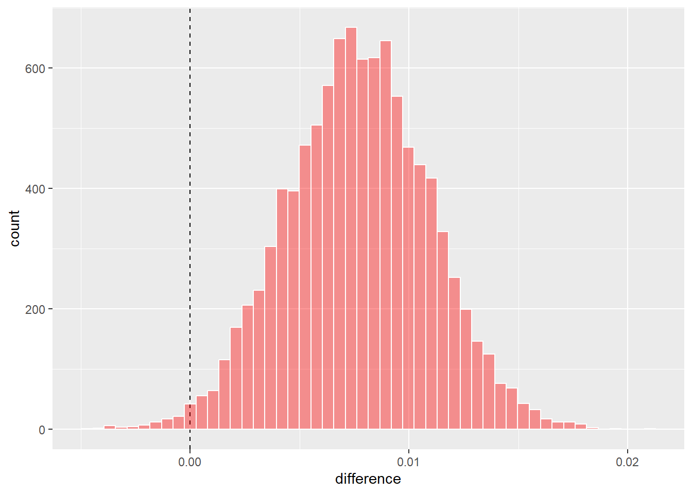
如 图 3.7 所示,不同模型之间的R2值差异的后验分布均值接近于0,且置信区间包含0,说明不同模型之间的R2值差异不具有统计学意义。可以进一步使用summary函数计算分布的平均值以及可信区间。其中,probability表示差异大于0的概率,mean表示差异的平均值。
代码
rsq_diff |>
  summary()
# A tibble: 1 × 9
contrast probability mean lower upper size pract_neg pract_equiv
<chr> <dbl> <dbl> <dbl> <dbl> <dbl> <dbl> <dbl>
1 splines_lm vs … 0.990 0.00768 0.00232 0.0130 0 NA NA
# ℹ 1 more variable: pract_pos <dbl>代码
rsq_anova |>
  autoplot(type = "ROPE", size = 0.02) +
  geom_text_repel(aes(label = workflow)) +
  theme(legend.position = "none")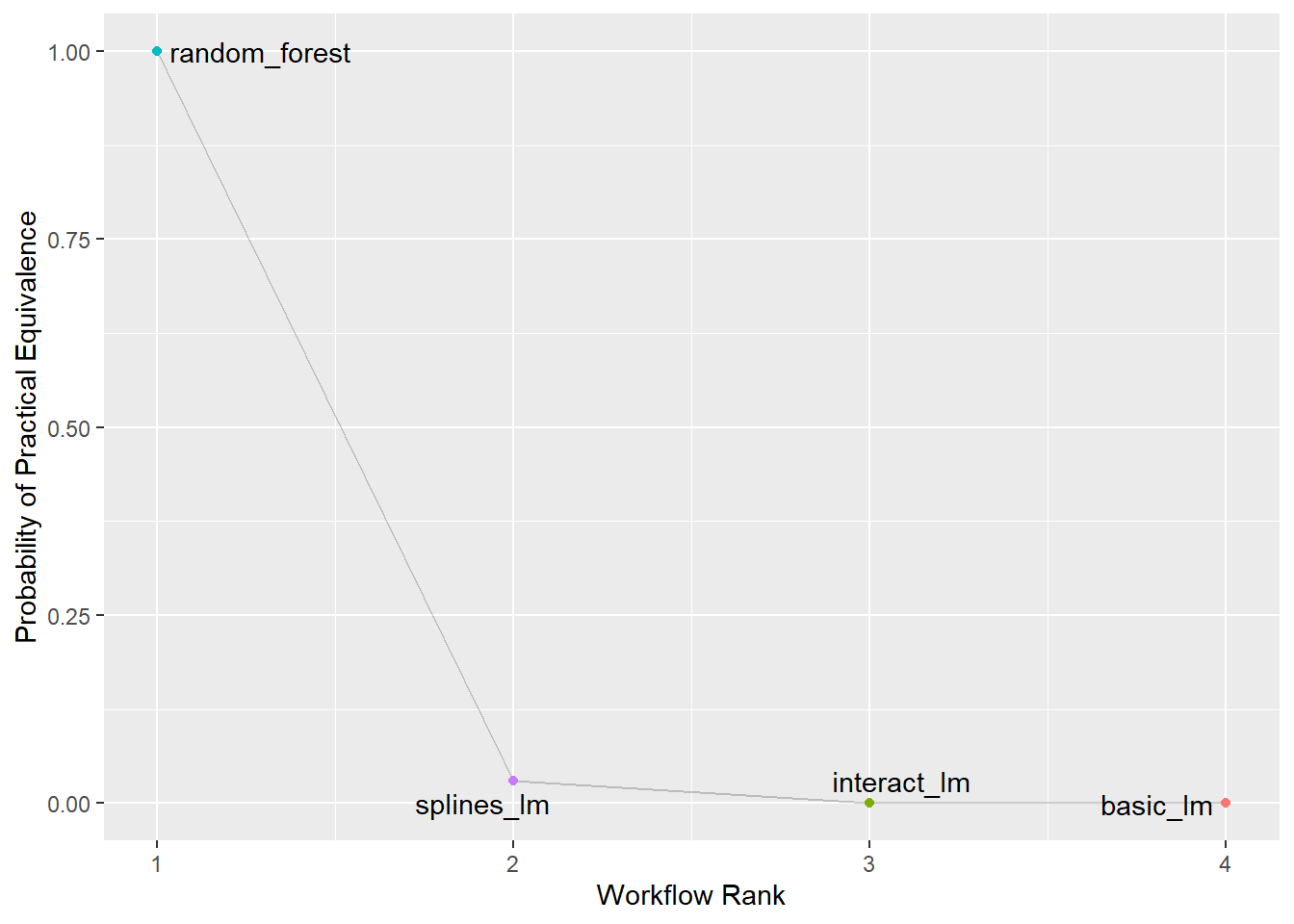
提示
重采样的次数越多,后验分布的形状越接近于正态分布。因此,可以通过增加重采样次数来提高模型的稳定性。