2 tidymodels-基础

作者

一把Fei刀

发布于

2024年2月5日

修改于

2025年2月1日

本篇是tidymodels包的学习笔记，主要参考文档是Tidy Modeling with R。

2.1 建模基础

---
title: 建模的分类
---
flowchart LR
A[模型] --- B[描述性模型]
A --- C[推理模型]
A --- D[预测模型]
D --- E[无监督模型]
D --- F[监督模型]
E --- G["主成分分析(PCA)"]
E --- H[聚类]
E --- I[自动编码器]
F --- J[回归]
F --- K[神经网络]

---
title: 模型建模的一般步骤
---
flowchart LR
A[导入数据] --> B["清洗数据(tidy)"] ---> C["探索性数据分析(EDA)"] --> D[特征工程] --> E[建模与优化] --> F[评估] --> G[部署]
F -.-> C

2.2 练习数据和探索性数据分析

练习数据使用的是modeldata包中的ames数据集。数据集包括：

房屋特征house characteristics，如bedrooms, garage, fireplace, pool, porch等；
区位location；
地块信息lot information，如zoning, shape, size等；
条件和质量评级ratings of condition and quality；
成交价格sale price。

代码

data(ames)
dim(ames)

[1] 2930   74

2.2.1 探索性数据分析-探索住宅特点

首先关注房屋的最终销售价格（美元）。使用直方图来查看销售价格的分布情况，如图 2.1 所示。

代码

tidymodels_prefer() # 用于处理包之间的函数冲突，不会输出结果

ames |>
  ggplot(aes(x = Sale_Price)) +
  geom_histogram(bins = 50, col = "white") +
  theme_bw() -> fig_0201

代码

fig_0201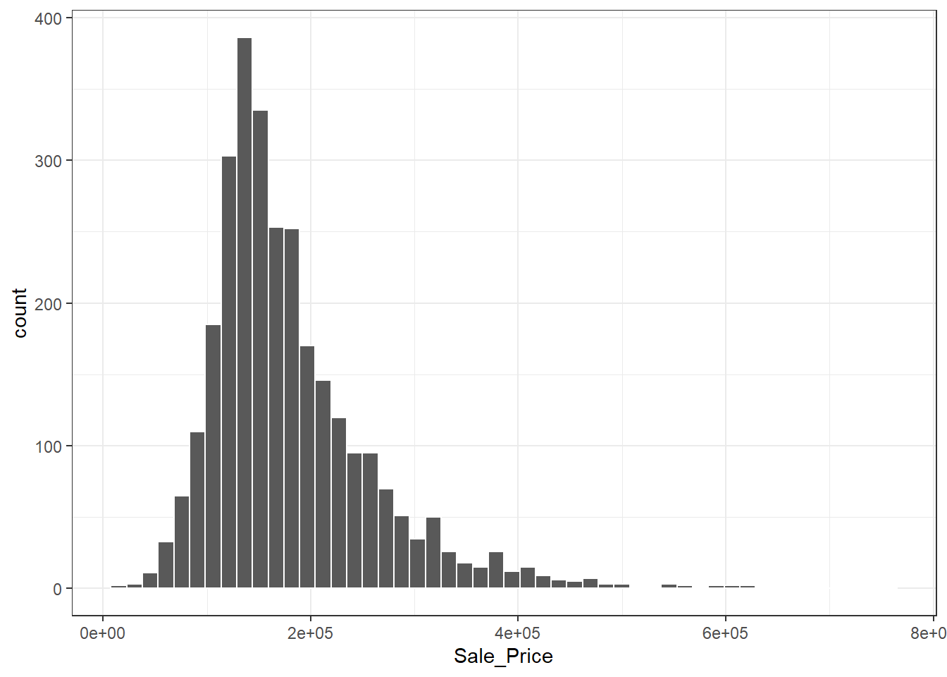

作图发现数据是偏态的，可以使用对数变换来处理。这种转换的优点是，不会预测出负销售价格的房屋，而且预测昂贵房屋的误差也不会对模型产生过大的影响。另外，对数变换还可以稳定方差，使得模型更容易拟合。结果如图 2.2 所示。

代码

fig_0201 +
  scale_x_log10() -> fig_0202

代码

fig_0202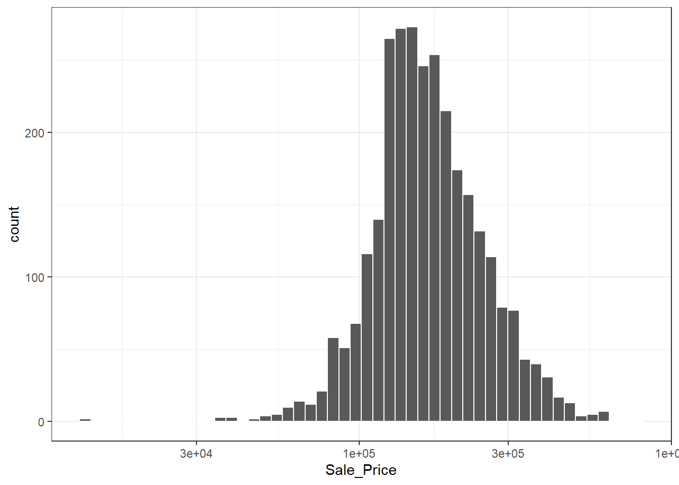

注意

对数转换结果的主要缺点涉及到对模型结果的解释。在对数变换后，模型的系数不再是直接解释的，而是对数解释。这意味着，模型的系数是对数销售价格的变化，而不是销售价格的变化。这种情况下，需要小心解释模型的结果。

对数转换的结果相对较好，因此可以使用对数转换后的销售价格作为目标变量。

代码

ames |>
  mutate(Sale_Price = log10(Sale_Price)) -> ames

2.3 数据分割

一般会将数据集分为训练集和测试集。训练集用于拟合模型，测试集用于评估模型的性能。

测试集只能使用一次，否则就会成为建模过程的一部分。这样会导致模型在测试集上的性能过于乐观，无法真实地评估模型的性能。

2.3.1 简单随机抽样

在tidymodels中，可以使用initial_split()函数来分割数据集。默认情况下，initial_split()函数会将数据集分为80%的训练集和20%的测试集。

代码

set.seed(123)

ames_split <- initial_split(ames, prop = 0.8)

ames_split

<Training/Testing/Total>
<2344/586/2930>

ames_split是一个rsplit对象，仅包含分区信息，可以使用training()和testing()函数来提取训练集和测试集。

代码

ames_train <- training(ames_split)
ames_test <- testing(ames_split)

dim(ames_train)

[1] 2344   74

2.3.2 分层抽样

在某些情况下，需要使用分层抽样。例如，如果数据集中有一个重要的类别变量，那么就需要使用分层抽样来确保训练集和测试集中都包含这个类别变量的各个水平。

可以人为地将结果数据四等分，然后分别进行四次分层抽样，这样可以保持训练集和测试集的分布一致。

代码

ames |>
  pull(Sale_Price) |> # 提取销售价格
  density(n = 2^10) |> # 生成密度估计
  tidy() -> sale_dens # 将结果转换为数据框

tibble(prob = (1:3)/4, value = quantile(ames$Sale_Price, probs = prob)) |> # 计算四分位数
  mutate(y = approx(sale_dens$x, sale_dens$y, xout = value)$y) -> quartiles # 计算四分位数的密度值

ames |>
  ggplot(aes(x = Sale_Price)) +
  geom_line(stat = "density") +
  geom_segment(data = quartiles,
               aes(x = value, xend = value, y = 0, yend = y),
               lty = 2) +
  labs(x = "Sale Price (log-10 USD)", y = NULL) +
  theme_bw() -> fig_0203
fig_0203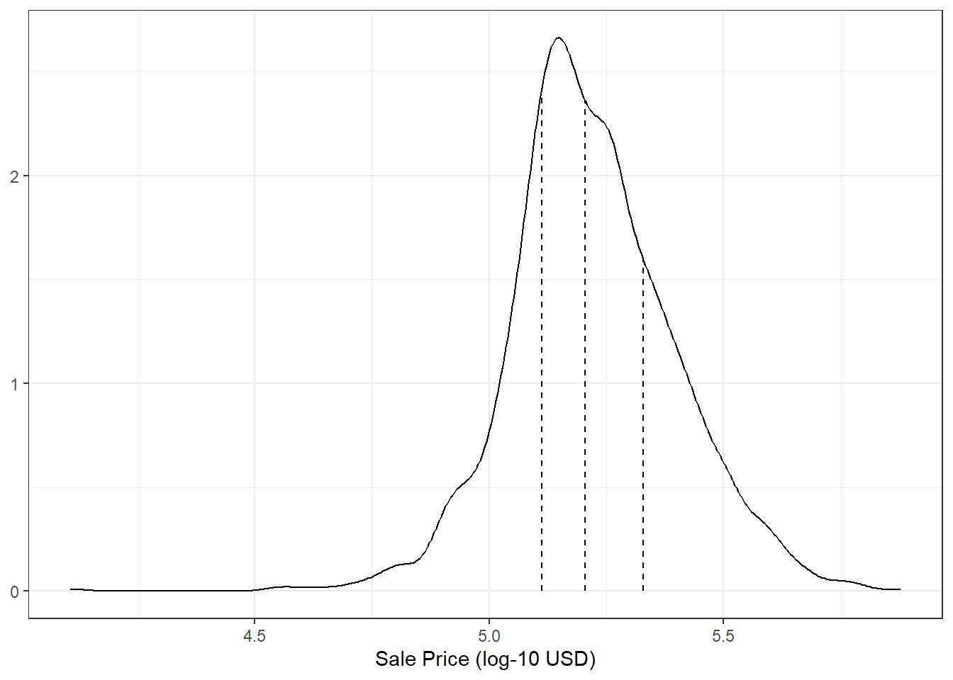

销售价格的分布呈右偏态，廉价房屋的比例更大。因此，可以使用分层抽样来确保训练集和测试集中都包含廉价房屋。可以使用strata参数来指定分层变量。

代码

set.seed(123)
ames_split <- initial_split(ames, prop = 0.80, strata = Sale_Price)
ames_train <- training(ames_split)
ames_test  <-  testing(ames_split)

dim(ames_train)

[1] 2342   74

注意

只能使用单列作为分层变量，不能使用多列。

2.3.3 交叉验证-验证集的分割

交叉验证通常用于解决模型过拟合的问题。为此，可以把数据集分为训练集、测试集和验证集，其中验证集用于调整模型的超参数。可以用initial_vadilation_split()函数来实现。

代码

set.seed(123)
ames_val_split <- initial_validation_split(ames, prop = c(0.6, 0.2))

ames_val_split

<Training/Validation/Testing/Total>
<1758/586/586/2930>

代码

ames_val_train <- training(ames_val_split)
ames_val_test  <- testing(ames_val_split)
ames_val_val   <- validation(ames_val_split)

2.4 模型拟合-以线性回归为例

对于一些相对简单的模型，可以使用parsnip包中的fit和predict函数来拟合和预测。parsnip包提供了统一的接口，可以使用相同的函数来拟合不同的模型。

使用parsnip中的linear_reg()函数指定模型类型，set_engine()函数指定模型引擎，这里的引擎一般指的是具体建模使用的软件包名称。确定模型后，可以使用fit()函数或fit_xy()函数来拟合模型。以三种常用的线性回归模型为例。

代码

linear_reg() |>
  set_engine("lm") |>
  translate()

Linear Regression Model Specification (regression)

Computational engine: lm 

Model fit template:
stats::lm(formula = missing_arg(), data = missing_arg(), weights = missing_arg())

代码

linear_reg(penalty = 1) |> # panalty是glmnet的特有参数
  set_engine("glmnet") |>
  translate()

Linear Regression Model Specification (regression)

Main Arguments:
  penalty = 1

Computational engine: glmnet 

Model fit template:
glmnet::glmnet(x = missing_arg(), y = missing_arg(), weights = missing_arg(), 
    family = "gaussian")

代码

linear_reg() |>
  set_engine("stan") |>
  translate()

Linear Regression Model Specification (regression)

Computational engine: stan 

Model fit template:
rstanarm::stan_glm(formula = missing_arg(), data = missing_arg(), 
    weights = missing_arg(), family = stats::gaussian, refresh = 0)

translate()函数可以提供模型转换的详细参数信息。
missing_arg()是占位符，表示数据未提供。

以经度和纬度为自变量，销售价格为因变量，拟合线性回归模型。

代码

linear_reg() |>
  set_engine("lm") -> lm_model

lm_model |>
  fit(Sale_Price ~ Longitude + Latitude, data = ames_train) -> lm_form_fit

lm_model |>
  fit_xy(x = ames_train |>
           select(Longitude, Latitude),
         y = ames_train |>
           pull(Sale_Price)
  ) -> lm_xy_fit

lm_form_fit

parsnip model object


Call:
stats::lm(formula = Sale_Price ~ Longitude + Latitude, data = data)

Coefficients:
(Intercept)    Longitude     Latitude  
   -300.251       -2.013        2.782

代码

lm_xy_fit

parsnip model object


Call:
stats::lm(formula = ..y ~ ., data = data)

Coefficients:
(Intercept)    Longitude     Latitude  
   -300.251       -2.013        2.782

2.5 提取模型结果

lm_form_fit和lm_xy_fit是parsnip模型对象，拟合模型储存在fit属性中。可以使用extract_fit_engine()函数提取拟合模型。

代码

lm_form_fit |>
  tidy() # 最简单的提取模型系数的方法（提取为tibble）

# A tibble: 3 × 5
  term        estimate std.error statistic  p.value
  <chr>          <dbl>     <dbl>     <dbl>    <dbl>
1 (Intercept)  -300.      14.6       -20.6 1.02e-86
2 Longitude      -2.01     0.130     -15.5 8.13e-52
3 Latitude        2.78     0.182      15.3 1.64e-50

代码

lm_form_fit |>
  extract_fit_engine() |> # 提取模型
  vcov() # 提取模型的协方差矩阵

            (Intercept)     Longitude      Latitude
(Intercept)  212.620590  1.6113032179 -1.4686377363
Longitude      1.611303  0.0168165968 -0.0008694728
Latitude      -1.468638 -0.0008694728  0.0330018995

代码

lm_form_fit |>
  extract_fit_engine() |>
  summary() |> # 提取模型的摘要信息
  coef() # 提取模型的系数

               Estimate Std. Error   t value     Pr(>|t|)
(Intercept) -300.250929 14.5815154 -20.59120 1.022609e-86
Longitude     -2.013413  0.1296788 -15.52615 8.126177e-52
Latitude       2.781713  0.1816642  15.31239 1.639312e-50

代码

lm_form_fit |>
  extract_fit_engine() |>
  gtsummary::tbl_regression() # 生成模型摘要信息

Characteristic	Beta	95% CI¹	p-value
Longitude	-2.0	-2.3, -1.8	<0.001
Latitude	2.8	2.4, 3.1	<0.001
¹ CI = Confidence Interval

2.6 模型预测

使用predict()函数进行预测。

代码

ames_test |>
  slice(1:5) -> ames_test_small # 选择前五行数据

predict(lm_form_fit, new_data = ames_test_small) # 预测结果

# A tibble: 5 × 1
  .pred
  <dbl>
1  5.22
2  5.22
3  5.28
4  5.24
5  5.31

代码

ames_test_small |>
  select(Sale_Price) |> # 真实值
  bind_cols(predict(lm_form_fit, ames_test_small)) |> # 预测值
  bind_cols(predict(lm_form_fit, ames_test_small, type = "pred_int")) # 预测区间

# A tibble: 5 × 4
  Sale_Price .pred .pred_lower .pred_upper
       <dbl> <dbl>       <dbl>       <dbl>
1       5.02  5.22        4.91        5.54
2       5.24  5.22        4.91        5.54
3       5.28  5.28        4.97        5.60
4       5.06  5.24        4.92        5.56
5       5.60  5.31        5.00        5.63

以决策树为例，对数据进行建模

代码

decision_tree(min_n = 2) |>
  set_engine("rpart") |>
  set_mode("regression") -> tree_model

tree_model |>
  fit(Sale_Price ~ Longitude + Latitude, data = ames_train) -> tree_fit

ames_test_small |>
  select(Sale_Price) |> # 真实值
  bind_cols(predict(tree_fit, ames_test_small)) # 预测值

# A tibble: 5 × 2
  Sale_Price .pred
       <dbl> <dbl>
1       5.02  5.15
2       5.24  5.15
3       5.28  5.31
4       5.06  5.15
5       5.60  5.52

重要

可以在https://www.tidymodels.org/find/找所有可用的模型。

parsnip_addin()函数可以在RStudio中搜索模型。

2.7 workflow

2.7.1 创建workflow对象

使用lm_model来创建workflow对象，workflow对象可以将数据预处理和模型拟合整合在一起。

代码

linear_reg() |>
  set_engine("lm") -> lm_model

代码

workflow() |>
  add_model(lm_model) -> lm_workflow

lm_workflow

══ Workflow ════════════════════════════════════════════════════════════════════
Preprocessor: None
Model: linear_reg()

── Model ───────────────────────────────────────────────────────────────────────
Linear Regression Model Specification (regression)

Computational engine: lm

注记

lm_workflow中，Preprocessor为空，代表没有数据预处理。

2.7.2 添加预处理器

使用add_formula函数输入标准公式作为预处理器：

代码

lm_workflow |>
  add_formula(Sale_Price ~ Longitude + Latitude) -> lm_workflow

lm_workflow

══ Workflow ════════════════════════════════════════════════════════════════════
Preprocessor: Formula
Model: linear_reg()

── Preprocessor ────────────────────────────────────────────────────────────────
Sale_Price ~ Longitude + Latitude

── Model ───────────────────────────────────────────────────────────────────────
Linear Regression Model Specification (regression)

Computational engine: lm

workflow对象可以使用fit()函数拟合模型，使用predict()函数进行预测。

代码

lm_workflow |>
  fit(data = ames_train) -> lm_fit

lm_fit

══ Workflow [trained] ══════════════════════════════════════════════════════════
Preprocessor: Formula
Model: linear_reg()

── Preprocessor ────────────────────────────────────────────────────────────────
Sale_Price ~ Longitude + Latitude

── Model ───────────────────────────────────────────────────────────────────────

Call:
stats::lm(formula = ..y ~ ., data = data)

Coefficients:
(Intercept)    Longitude     Latitude  
   -300.251       -2.013        2.782

代码

lm_fit |>
  predict(new_data = ames_test |>
            slice(1:3)) # 预测

# A tibble: 3 × 1
  .pred
  <dbl>
1  5.22
2  5.22
3  5.28

可以使用update_formula函数更新预处理器：

代码

lm_fit |>
  update_formula(Sale_Price ~ Longitude)

══ Workflow ════════════════════════════════════════════════════════════════════
Preprocessor: Formula
Model: linear_reg()

── Preprocessor ────────────────────────────────────────────────────────────────
Sale_Price ~ Longitude

── Model ───────────────────────────────────────────────────────────────────────
Linear Regression Model Specification (regression)

Computational engine: lm

2.7.3 添加变量

使用add_variables函数添加变量。函数有两个参数：outcomes和predictors。支持使用c()函数添加多个变量。

代码

lm_workflow |>
  remove_formula() |>
  add_variables(outcome = Sale_Price, predictors = c(Longitude, Latitude)) -> lm_workflow # 和上面的add_formula等价

lm_workflow

══ Workflow ════════════════════════════════════════════════════════════════════
Preprocessor: Variables
Model: linear_reg()

── Preprocessor ────────────────────────────────────────────────────────────────
Outcomes: Sale_Price
Predictors: c(Longitude, Latitude)

── Model ───────────────────────────────────────────────────────────────────────
Linear Regression Model Specification (regression)

Computational engine: lm

拟合模型：

代码

fit(lm_workflow, data = ames_train) # 拟合模型

══ Workflow [trained] ══════════════════════════════════════════════════════════
Preprocessor: Variables
Model: linear_reg()

── Preprocessor ────────────────────────────────────────────────────────────────
Outcomes: Sale_Price
Predictors: c(Longitude, Latitude)

── Model ───────────────────────────────────────────────────────────────────────

Call:
stats::lm(formula = ..y ~ ., data = data)

Coefficients:
(Intercept)    Longitude     Latitude  
   -300.251       -2.013        2.782

2.7.4 为`workflow`使用公式

2.7.4.1 基于树的模型

使用Orthodont数据集，拟合一个受试者具有随机效应的回归模型。

在workflow中，使用add_variables()函数添加变量，使用add_model()函数添加模型。

代码

library(multilevelmod) # parsnip扩展包，主要用于多层次模型（混合效应模型、贝叶斯层次模型等）

data(Orthodont, package = "nlme")

linear_reg() |>
  set_engine("lmer") -> multilevel_spec # lmer是lme4包中的函数，用于拟合线性混合效应模型

workflow() |>
  add_variables(outcome = distance, predictors = c(Sex, age, Subject)) |>
  add_model(multilevel_spec,
            formula = distance ~ Sex + (age | Subject)) -> multilevel_workflow # age | Subject表示age是Subject的随机效应

multilevel_workflow |>
  fit(data = Orthodont) -> multilevel_fit

multilevel_fit

══ Workflow [trained] ══════════════════════════════════════════════════════════
Preprocessor: Variables
Model: linear_reg()

── Preprocessor ────────────────────────────────────────────────────────────────
Outcomes: distance
Predictors: c(Sex, age, Subject)

── Model ───────────────────────────────────────────────────────────────────────
Linear mixed model fit by REML ['lmerMod']
Formula: distance ~ Sex + (age | Subject)
   Data: data
REML criterion at convergence: 471.1635
Random effects:
 Groups   Name        Std.Dev. Corr 
 Subject  (Intercept) 7.3912        
          age         0.6943   -0.97
 Residual             1.3100        
Number of obs: 108, groups:  Subject, 27
Fixed Effects:
(Intercept)    SexFemale  
     24.517       -2.145

可以进一步使用survival包中的strata函数进行生存分析.

代码

library(censored) # parsnip扩展包，主要用于删减回归和生存分析模型

survival_reg() -> parametric_spec

data(cancer, package = "survival")

workflow() |>
  add_variables(outcome = c(fustat, futime), predictors = c(age, rx)) |>
  add_model(parametric_spec,
            formula = Surv(futime, fustat) ~ age + strata(rx)) -> parametric_workflow

parametric_workflow |>
  fit(data = ovarian) -> parametric_fit

parametric_fit

══ Workflow [trained] ══════════════════════════════════════════════════════════
Preprocessor: Variables
Model: survival_reg()

── Preprocessor ────────────────────────────────────────────────────────────────
Outcomes: c(fustat, futime)
Predictors: c(age, rx)

── Model ───────────────────────────────────────────────────────────────────────
Call:
survival::survreg(formula = Surv(futime, fustat) ~ age + strata(rx), 
    data = data, model = TRUE)

Coefficients:
(Intercept)         age 
 12.8734120  -0.1033569 

Scale:
     rx=1      rx=2 
0.7695509 0.4703602 

Loglik(model)= -89.4   Loglik(intercept only)= -97.1
    Chisq= 15.36 on 1 degrees of freedom, p= 8.88e-05 
n= 26

2.7.5 同时创建多个workflow

做预测模型时，一般需要评估多个不同的模型。例如筛选预测因子。可以创建一组formula来罗列不同的预测因子组合。

代码

list(
  longitude = Sale_Price ~ Longitude,
  latitude = Sale_Price ~ Latitude,
  coords = Sale_Price ~ Longitude + Latitude,
  neighborhood = Sale_Price ~ Neighborhood) -> location

使用workflow_set()函数创建一个workflow集合。

代码

workflow_set(preproc = location, models = list(lm = lm_model)) -> location_models

location_models

# A workflow set/tibble: 4 × 4
  wflow_id        info             option    result    
  <chr>           <list>           <list>    <list>    
1 longitude_lm    <tibble [1 × 4]> <opts[0]> <list [0]>
2 latitude_lm     <tibble [1 × 4]> <opts[0]> <list [0]>
3 coords_lm       <tibble [1 × 4]> <opts[0]> <list [0]>
4 neighborhood_lm <tibble [1 × 4]> <opts[0]> <list [0]>

代码

location_models$info[[1]] # 查看第一个workflow的信息

# A tibble: 1 × 4
  workflow   preproc model      comment
  <list>     <chr>   <chr>      <chr>  
1 <workflow> formula linear_reg ""

代码

extract_workflow(location_models, id = "coords_lm") # 提取一个workflow

══ Workflow ════════════════════════════════════════════════════════════════════
Preprocessor: Formula
Model: linear_reg()

── Preprocessor ────────────────────────────────────────────────────────────────
Sale_Price ~ Longitude + Latitude

── Model ───────────────────────────────────────────────────────────────────────
Linear Regression Model Specification (regression)

Computational engine: lm

为每个formula创建fit对象：

代码

location_models |>
  mutate(fit = map(info, ~ fit(.x$workflow[[1]], ames_train))) -> location_models # 使用map函数对每个workflow进行拟合

location_models

# A workflow set/tibble: 4 × 5
  wflow_id        info             option    result     fit       
  <chr>           <list>           <list>    <list>     <list>    
1 longitude_lm    <tibble [1 × 4]> <opts[0]> <list [0]> <workflow>
2 latitude_lm     <tibble [1 × 4]> <opts[0]> <list [0]> <workflow>
3 coords_lm       <tibble [1 × 4]> <opts[0]> <list [0]> <workflow>
4 neighborhood_lm <tibble [1 × 4]> <opts[0]> <list [0]> <workflow>

代码

location_models$fit[[1]] # 查看第一个workflow的拟合结果

══ Workflow [trained] ══════════════════════════════════════════════════════════
Preprocessor: Formula
Model: linear_reg()

── Preprocessor ────────────────────────────────────────────────────────────────
Sale_Price ~ Longitude

── Model ───────────────────────────────────────────────────────────────────────

Call:
stats::lm(formula = ..y ~ ., data = data)

Coefficients:
(Intercept)    Longitude  
    -176.46        -1.94

2.7.6 评估测试集

使用last_fit函数，可以把模型拟合到整个训练集，然后评估测试集。

代码

last_fit(lm_workflow, ames_split) -> final_lm_res # 用法：last_fit(模型, 数据分割)

final_lm_res

# Resampling results
# Manual resampling 
# A tibble: 1 × 6
  splits             id               .metrics .notes   .predictions .workflow 
  <list>             <chr>            <list>   <list>   <list>       <list>    
1 <split [2342/588]> train/test split <tibble> <tibble> <tibble>     <workflow>

代码

final_lm_res |>
  extract_workflow() # 提取workflow

══ Workflow [trained] ══════════════════════════════════════════════════════════
Preprocessor: Variables
Model: linear_reg()

── Preprocessor ────────────────────────────────────────────────────────────────
Outcomes: Sale_Price
Predictors: c(Longitude, Latitude)

── Model ───────────────────────────────────────────────────────────────────────

Call:
stats::lm(formula = ..y ~ ., data = data)

Coefficients:
(Intercept)    Longitude     Latitude  
   -300.251       -2.013        2.782

代码

final_lm_res |>
  collect_metrics() # 收集模型评估指标

# A tibble: 2 × 4
  .metric .estimator .estimate .config             
  <chr>   <chr>          <dbl> <chr>               
1 rmse    standard       0.160 Preprocessor1_Model1
2 rsq     standard       0.208 Preprocessor1_Model1

代码

final_lm_res |>
  collect_predictions() |> # 收集预测结果
  head()

# A tibble: 6 × 5
  .pred id                .row Sale_Price .config             
  <dbl> <chr>            <int>      <dbl> <chr>               
1  5.22 train/test split     2       5.02 Preprocessor1_Model1
2  5.22 train/test split     3       5.24 Preprocessor1_Model1
3  5.28 train/test split     5       5.28 Preprocessor1_Model1
4  5.24 train/test split    28       5.06 Preprocessor1_Model1
5  5.31 train/test split    39       5.60 Preprocessor1_Model1
6  5.31 train/test split    44       5.33 Preprocessor1_Model1

2.8 特征工程

特征工程指对预测值进行重新格式化，使其更容易被模型有效利用。特征工程的方法一般分为以下几种：

dummy，哑变量，将分类变量分为多个哑变量（0-1变量）。
zv， zero variance，删除方差为0的变量，也就是只有单一值的变量。
impute，估算，填补缺失值。
decorrelate，去相关，删除相关性较高的变量。一般使用PCA方法或者VIF方法。
normalize，标准化，将变量居中并缩放到单位方差。
transform，转换，将变量转换成更对称的分布。

使用recipe包可以把不同的特征工程方法组合在一起，并应用到数据集上。

2.8.1 创建特征工程

从ames数据集中挑选以下预测因子：

Neighborhood，分类变量，指房屋所在的社区，有29个水平。
Gr_Liv_Area，数值变量，指房屋的居住面积。
Year_Built，数值变量，指房屋建造的年份。
Bldg_Type，分类变量，指房屋的类型，有5个水平，分别是OneFam，TwoFmCon，Duplex，Twnhs，TwnhsE。

使用这些预测因子对Sale_Price进行预测，公式如下：

代码

lm(Sale_Price ~ Neighborhood + log10(Gr_Liv_Area) + Year_Built + Bldg_Type, data = ames) # 由于Sale_Price取过对数，所以Gr_Liv_Area也取对数

根据预测因子的性质和上述公式，使用recipe创建一个特征工程流程。

代码

recipe(Sale_Price ~ Neighborhood + Gr_Liv_Area + Year_Built + Bldg_Type,
       data = ames) |> # 创建recipe对象，声明结果变量和预测因子
  step_log(Gr_Liv_Area) |> # 对Gr_Liv_Area取对数
  step_dummy(all_nominal_predictors()) -> simple_ames # 对分类变量创建哑变量

simple_ames

提示

all_nominal_predictors()函数用于选择所有的分类变量。

all_numeric_predictors()函数用于选择所有的数值变量。

all_predictors()函数用于选择所有的预测因子。

all_outcomes()函数用于选择所有的结果变量。

all_numeric()函数用于选择所有的数值变量。

2.8.2 应用特征工程

将特征工程simple_ames应用到workflowlm_workflow上。

代码

lm_workflow |>
  remove_variables() |> # 删除所有的预测因子
  remove_recipe() |> # 删除所有的特征工程
  add_recipe(simple_ames) -> lm_workflow # 添加特征工程

lm_workflow

══ Workflow ════════════════════════════════════════════════════════════════════
Preprocessor: Recipe
Model: linear_reg()

── Preprocessor ────────────────────────────────────────────────────────────────
2 Recipe Steps

• step_log()
• step_dummy()

── Model ───────────────────────────────────────────────────────────────────────
Linear Regression Model Specification (regression)

Computational engine: lm

代码

fit(lm_workflow, ames_train) -> lm_fit # 拟合模型

predict(lm_fit, ames_test) |> # 预测测试集
  head()

# A tibble: 6 × 1
  .pred
  <dbl>
1  5.07
2  5.17
3  5.27
4  5.08
5  5.51
6  5.44

使用extract_*函数可以提取fit对象的不同信息，如模型参数、特征工程等。

代码

lm_fit |>
  extract_recipe(estimated = TRUE) # 提取特征工程，estimated = TRUE表示提取特征工程的估计值

lm_fit |>
  extract_fit_parsnip() |> # 提取模型参数
  tidy() |>
  head()

# A tibble: 6 × 5
  term                       estimate std.error statistic   p.value
  <chr>                         <dbl>     <dbl>     <dbl>     <dbl>
1 (Intercept)                -0.682    0.228        -2.99 2.78e-  3
2 Gr_Liv_Area                 0.271    0.00606      44.8  1.36e-315
3 Year_Built                  0.00199  0.000115     17.3  6.19e- 63
4 Neighborhood_College_Creek  0.0167   0.00807       2.06 3.91e-  2
5 Neighborhood_Old_Town      -0.0357   0.00844      -4.22 2.50e-  5
6 Neighborhood_Edwards       -0.0531   0.00755      -7.04 2.57e- 12

2.8.3 其他特征工程示例

2.8.3.1 定性变量的处理

提示

step_unknown()函数用于将缺失值转化为专用因子水平。

step_novel()函数用于将未知的水平转化为新的水平。

step_other()函数用于将频率较低的多个水平合并为一个水平，频率阈值可以指定。

上述函数可以用于处理定性变量的缺失值和未知水平，以及合并频率较低的水平，在此基础上，可以使用step_dummy()函数创建哑变量。

2.8.3.2 交互项的处理

交互项是指两个或多个变量的乘积，可以用于捕捉变量之间的关系。使用step_interact(~*:*)函数可以创建交互项。

在ames数据集中，不同建筑类型的房屋可能与不同的居住面积存在交互，如图 2.4 所示，可以使用交互项来捕捉这种关系。

代码

ggplot(ames_train, aes(x = Gr_Liv_Area, y = 10^Sale_Price)) +
  geom_point(alpha = .2) +
  facet_wrap(~ Bldg_Type) +
  geom_smooth(method = lm, formula = y ~ x, se = FALSE, color = "lightblue") +
  scale_x_log10() +
  scale_y_log10() +
  labs(x = "Gross Living Area", y = "Sale Price (USD)")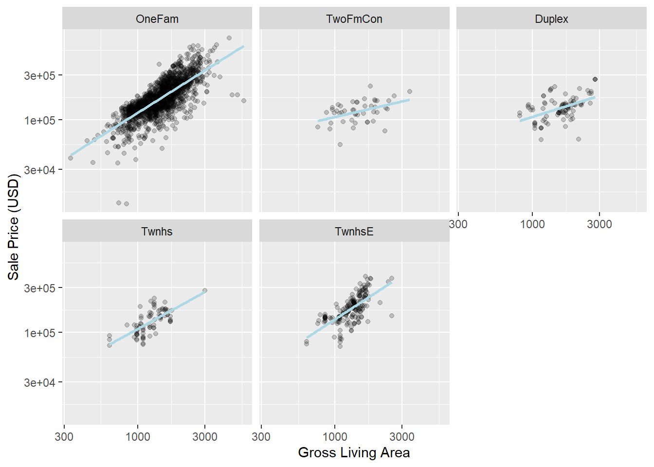

代码

recipe(Sale_Price ~ Neighborhood + Gr_Liv_Area + Year_Built + Bldg_Type,
         data = ames_train) |> # 创建recipe对象并声明结果变量和预测因子
  step_log(Gr_Liv_Area, base = 10) |> # 对Gr_Liv_Area取对数
  step_other(Neighborhood, threshold = 0.01) |> # 合并频率较低的水平
  step_dummy(all_nominal_predictors()) |> # 对分类变量创建哑变量
  step_interact( ~ Gr_Liv_Area:starts_with("Bldg_Type_")) -> simple_ames # 创建交互项，其中:表示交互，可以使用+添加多组交互项

simple_ames

警告

一般来说，交互项需要在创建哑变量后才能创建，否则可能会报错。

2.8.3.3 样条函数

样条函数是一种非参数拟合方法，可以用于拟合非线性关系。使用step_ns()函数可以创建样条函数。

在ames数据集中，经度和纬度可能与销售价格存在非线性关系，如图 2.5 所示，可以使用样条函数来捕捉这种关系。

代码

library(splines) # 样条函数
library(patchwork) # 绘图拼接

plot_smoother <- function(deg_free) { # 创建一个函数，用于绘制不同自由度的样条函数
  ggplot(ames_train, aes(x = Latitude, y = 10^Sale_Price)) +  # 还原对数变换
    geom_point(alpha = .2) +  # 添加散点图，alpha表示透明度
    scale_y_log10() + # 对y轴进行对数变换
    geom_smooth(
      method = lm,
      formula = y ~ ns(x, df = deg_free),
      color = "lightblue",
      se = FALSE
    ) + # 添加样条函数，ns表示样条函数，df表示自由度
    labs(title = paste(deg_free, "Spline Terms"),
         y = "Sale Price (USD)")
}

( plot_smoother(2) + plot_smoother(5) ) / ( plot_smoother(20) + plot_smoother(100) ) # 绘制不同自由度的样条函数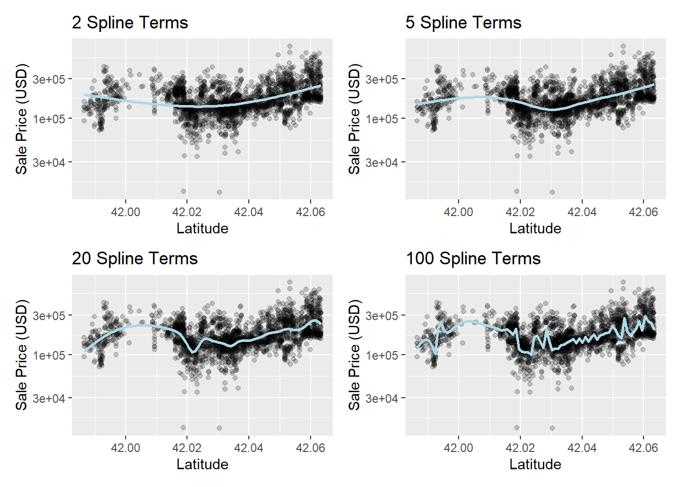

由图 2.5 可以看出，自由度为5和20时，样条函数能较好地拟合数据，这里选择自由度为20的样条函数来捕捉纬度与销售价格的关系。

代码

recipe(Sale_Price ~ Neighborhood + Gr_Liv_Area + Year_Built + Bldg_Type + Latitude,
         data = ames_train) |>
  step_log(Gr_Liv_Area, base = 10) |>
  step_other(Neighborhood, threshold = 0.01) |>
  step_dummy(all_nominal_predictors()) %>%
  step_interact( ~ Gr_Liv_Area:starts_with("Bldg_Type_") ) |>
  step_ns(Latitude, deg_free = 20) # 创建样条函数，自由度为20

2.8.3.4 特征提取（PCA）

特征提取是指将多个原始特征合并为少数几个新特征，以减少数据维度。使用step_pca()函数可以进行主成分分析（PCA）。

PCA是一种线性提取方法，其优点是每个主成分之间互不相关，因此可以减少多重共线性的影响。但是，PCA的缺点是提取的特征不易解释，而且新特征可能与结果无关。

在ames数据集中，有几个预测因子测量了房产的面积，如地下室总面积Total_Bsmt_SF、一楼面积First_Flr_SF、总居住面积Gr_Liv_Area等。PCA 可以将这些潜在的冗余变量表示为一个较小的特征集。除了总居住面积外，这些预测因子的名称中都有后缀SF（表示平方英尺）。

PCA假定所有预测因子的单位相同，因此在使用PCA之前，最好使用step_normalize()对这些预测因子进行标准化。

代码

step_normalize(matches("(SF$)|(Gr_Liv)")) |>
step_pca(matches("(SF$)|(Gr_Liv)"))

提示

特征提取的其他方法还包括独立成分分析（ICA），非负矩阵分解（NMF），多维缩放（MDS），均匀流形近似（UMAP），t-分布邻域嵌入（t-SNE）等。

2.8.3.5 抽样技术

类别不平衡问题是指分类问题中不同类别的样本数量差异较大。在这种情况下，模型可能会偏向于预测样本数量较多的类别，而忽略样本数量较少的类别。针对类别不平衡问题，可以采用子采样技术，它通常不会提高整体性能，但可以生成表现更好的预测类概率分布。子采样技术分类如下：

下抽样(Downsampling)：保留少数类样本，对多数类样本进行随机抽样，以平衡频率。
扩大抽样(Upsampling)：合成新的少数类样本，或直接复制少数类样本，以平衡频率。
Hybrid：结合上述两种方法。

在themis包中，step_downsample()和step_upsample()函数可以实现下抽样和扩大抽样。

提示

step_filter()函数可以用于删除不需要的样本，如异常值、缺失值等。

step_sample()函数可以用于随机抽样。

step_slice()函数可以用于分割数据集。

step_arrange()函数可以用于排序数据集。

2.8.3.6 一般变换

一般变换是指对数据进行一般性的变换，如对数变换、幂变换、指数变换等。在recipes包中，step_log()、step_sqrt()、step_YeoJohnson()、step_boxcox()等函数可以实现对数变换、平方根变换、Yeo-Johnson变换、Box-Cox变换等。step_mutate()函数可以利用已有变量计算并创建新的变量。

警告

进行一般变换是，需要格外注意避免数据泄露。转换应该在拆分数据集之前进行。

2.8.3.7 自然语言处理

自然语言处理（NLP）是指对文本数据进行处理，如分词、词干提取、词形还原、停用词过滤、词频统计、TF-IDF计算等。

textrecipes包是recipes包的扩展，提供了一系列用于文本数据处理的函数。step_tokenize()、step_stem()、step_lemma()、step_stopwords()、step_tf()、step_tfidf()等函数可以实现分词、词干提取、词形还原、停用词过滤、词频统计、TF-IDF计算等。可以在Cookbook - Using more complex recipes involving text中参考相关函数的使用方法。但是，textrecipes包目前还不支持中文文本的处理，可能需要使用jiebaR包（jiebaR 中文分词文档）等其他包来处理中文文本。

2.8.4 tidy

首先，为ames数据集创建一个recipe对象。然后，使用tidy()函数查看recipe对象的内容摘要。

id参数可以用于指定recipe步骤函数的标识符。在多次添加相同的步骤函数时，可以使用id参数来区分这些步骤函数。

代码

recipe(Sale_Price ~ Neighborhood + Gr_Liv_Area + Year_Built + Bldg_Type +
         Latitude + Longitude, data = ames_train) |>
  step_log(Gr_Liv_Area, base = 10) |>
  step_other(Neighborhood, threshold = 0.01, id = "my_id") |> # 指定id参数
  step_dummy(all_nominal_predictors()) |>
  step_interact( ~ Gr_Liv_Area:starts_with("Bldg_Type_")) |>
  step_ns(Latitude, Longitude, deg_free = 20) -> ames_recipe

ames_recipe |>
  tidy()

# A tibble: 5 × 6
  number operation type     trained skip  id            
   <int> <chr>     <chr>    <lgl>   <lgl> <chr>         
1      1 step      log      FALSE   FALSE log_yQoQt     
2      2 step      other    FALSE   FALSE my_id         
3      3 step      dummy    FALSE   FALSE dummy_EvyKp   
4      4 step      interact FALSE   FALSE interact_VANTp
5      5 step      ns       FALSE   FALSE ns_J20uP

使用ames_recipe对象建立workflow：

代码

workflow() |>
  add_model(lm_model) |>
  add_recipe(ames_recipe) -> lm_workflow

lm_workflow |>
  fit(data = ames_train) -> lm_fit

可以使用tidy()函数并指定id参数，查看对应id步骤的结果，也可以指定number参数，查看对应的结果：

代码

lm_fit |>
  extract_recipe(estimated = TRUE) |>
  tidy(id = "my_id")

# A tibble: 21 × 3
   terms        retained           id   
   <chr>        <chr>              <chr>
 1 Neighborhood North_Ames         my_id
 2 Neighborhood College_Creek      my_id
 3 Neighborhood Old_Town           my_id
 4 Neighborhood Edwards            my_id
 5 Neighborhood Somerset           my_id
 6 Neighborhood Northridge_Heights my_id
 7 Neighborhood Gilbert            my_id
 8 Neighborhood Sawyer             my_id
 9 Neighborhood Northwest_Ames     my_id
10 Neighborhood Sawyer_West        my_id
# ℹ 11 more rows

代码

lm_fit |>
  extract_recipe(estimated = TRUE) |>
  tidy(number = 3)

# A tibble: 25 × 3
   terms        columns            id         
   <chr>        <chr>              <chr>      
 1 Neighborhood College_Creek      dummy_EvyKp
 2 Neighborhood Old_Town           dummy_EvyKp
 3 Neighborhood Edwards            dummy_EvyKp
 4 Neighborhood Somerset           dummy_EvyKp
 5 Neighborhood Northridge_Heights dummy_EvyKp
 6 Neighborhood Gilbert            dummy_EvyKp
 7 Neighborhood Sawyer             dummy_EvyKp
 8 Neighborhood Northwest_Ames     dummy_EvyKp
 9 Neighborhood Sawyer_West        dummy_EvyKp
10 Neighborhood Mitchell           dummy_EvyKp
# ℹ 15 more rows

2.8.5 “roles”变量

有一部分变量，既不是预测变量，也不是因子变量，但在数据集中可能起到建模之外的作用。可以使用add_role(), remove_role()和update_role()函数来指定这些变量的角色。同时，可以为step_*()函数指定roles参数，不过大部分step_*()函数都会自动给定变量的角色。

代码示例：

代码

ames_recipe |>
  update_role(address, new_role = "street address") # 对于已建好的recipe对象，使用update_role()函数来更新变量的角色，在构建recipe对象时，应使用add_role()函数。

2.9 模型性能评估

重要

重采样方法是最有效的验证方法。

yardstick包是tidymodels核心包之一，可以用于模型性能评估。按结果变量的类型，即数值变量、二分类变量和多分类变量，模型性能评估的指标也有所不同。

2.9.1 数值变量-回归模型

ames数据集的预测模型lm_fit包含了回归模型和预测集，同时有交互作用和经纬度样条函数。首先，使用predict()函数计算预测值。

代码

lm_fit |>
  predict(new_data = ames_test |>
            select(-Sale_Price)) -> ames_test_results

ames_test_results |>
  head()

# A tibble: 6 × 1
  .pred
  <dbl>
1  5.07
2  5.17
3  5.28
4  5.05
5  5.51
6  5.42

将预测值和实际值放在一起，使用bind_cols()函数：

代码

ames_test_results |>
  bind_cols(ames_test |>
              select(Sale_Price)) -> ames_test_results

ames_test_results |>
  head()

# A tibble: 6 × 2
  .pred Sale_Price
  <dbl>      <dbl>
1  5.07       5.02
2  5.17       5.24
3  5.28       5.28
4  5.05       5.06
5  5.51       5.60
6  5.42       5.33

首先，作图查看预测值和实际值的关系：

代码

ggplot(ames_test_results, aes(x = Sale_Price, y = .pred)) +
  geom_abline(lty = 2) + # 添加对角线
  geom_point(alpha = 0.5) +
  labs(y = "Predicted Sale Price (log10)", x = "Sale Price (log10)") +
  coord_obs_pred() # 使x轴和y轴的刻度一致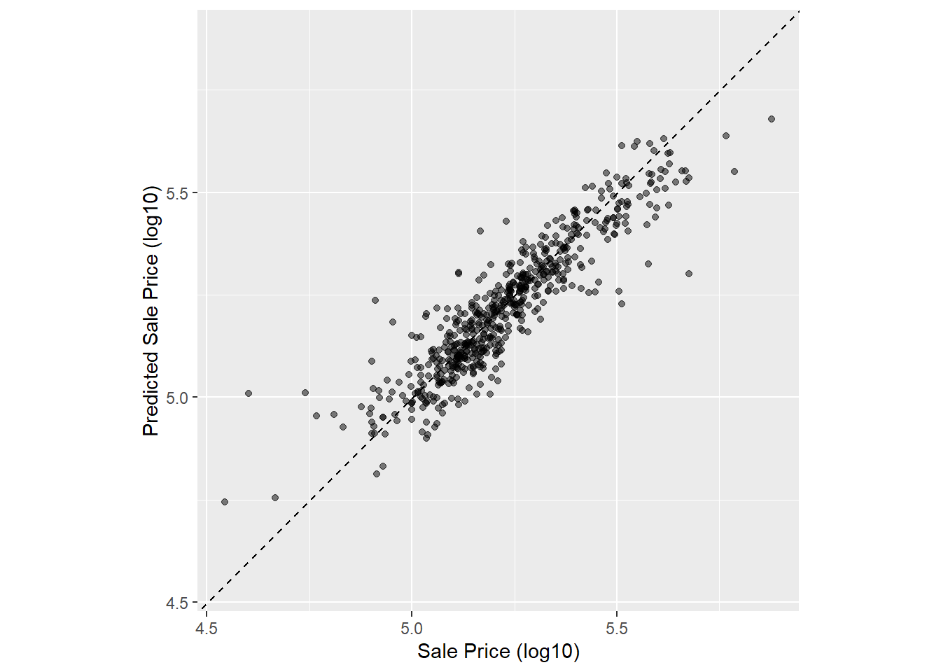

由图 2.6 发现，有几个预测值和实际值的偏差较大。使用rmse()函数计算均方根误差，rsq函数计算R^2，mae函数计算平均绝对误差。

代码

ames_test_results |>
  rmse(truth = Sale_Price, estimate = .pred) # 计算单一指标

# A tibble: 1 × 3
  .metric .estimator .estimate
  <chr>   <chr>          <dbl>
1 rmse    standard      0.0754

代码

ames_metrics <- metric_set(rmse, rsq, mae) # 创建指标集

ames_test_results |>
  ames_metrics(truth = Sale_Price, estimate = .pred) # 同时计算多个指标

# A tibble: 3 × 3
  .metric .estimator .estimate
  <chr>   <chr>          <dbl>
1 rmse    standard      0.0754
2 rsq     standard      0.826 
3 mae     standard      0.0546

2.9.2 二分类变量-logistic回归模型

使用modeldata包（tidymodels核心包之一）中的two_class_example数据集，这是一个模拟了logistic回归模型预测结果的数据集。

代码

data(two_class_example, package = "modeldata")
tibble(two_class_example) |>
  head()

# A tibble: 6 × 4
  truth   Class1   Class2 predicted
  <fct>    <dbl>    <dbl> <fct>    
1 Class2 0.00359 0.996    Class2   
2 Class1 0.679   0.321    Class1   
3 Class2 0.111   0.889    Class2   
4 Class1 0.735   0.265    Class1   
5 Class2 0.0162  0.984    Class2   
6 Class1 0.999   0.000725 Class1

对于logistic回归模型，模型性能评估指标有很多，列举如下：

conf_mat：混淆矩阵

代码

two_class_example |>
  conf_mat(truth = truth, estimate = predicted)

          Truth
Prediction Class1 Class2
    Class1    227     50
    Class2     31    192

accuracy：准确率

代码

two_class_example |>
  accuracy(truth = truth, estimate = predicted)

# A tibble: 1 × 3
  .metric  .estimator .estimate
  <chr>    <chr>          <dbl>
1 accuracy binary         0.838

mcc：Matthews相关系数

代码

two_class_example |>
  mcc(truth = truth, estimate = predicted)

# A tibble: 1 × 3
  .metric .estimator .estimate
  <chr>   <chr>          <dbl>
1 mcc     binary         0.677

f_meas：F1值，精确率和召回率的调和平均数

代码

two_class_example |>
  f_meas(truth = truth, estimate = predicted)

# A tibble: 1 × 3
  .metric .estimator .estimate
  <chr>   <chr>          <dbl>
1 f_meas  binary         0.849

roc_curve和roc_auc：ROC曲线和AUC

代码

two_class_example |>
  roc_curve(truth = truth, Class1) -> two_class_curve

two_class_curve

# A tibble: 502 × 3
   .threshold specificity sensitivity
        <dbl>       <dbl>       <dbl>
 1 -Inf           0                 1
 2    1.79e-7     0                 1
 3    4.50e-6     0.00413           1
 4    5.81e-6     0.00826           1
 5    5.92e-6     0.0124            1
 6    1.22e-5     0.0165            1
 7    1.40e-5     0.0207            1
 8    1.43e-5     0.0248            1
 9    2.38e-5     0.0289            1
10    3.30e-5     0.0331            1
# ℹ 492 more rows

代码

two_class_example |>
  roc_auc(truth = truth, Class1)

# A tibble: 1 × 3
  .metric .estimator .estimate
  <chr>   <chr>          <dbl>
1 roc_auc binary         0.939

代码

two_class_curve |>
  autoplot()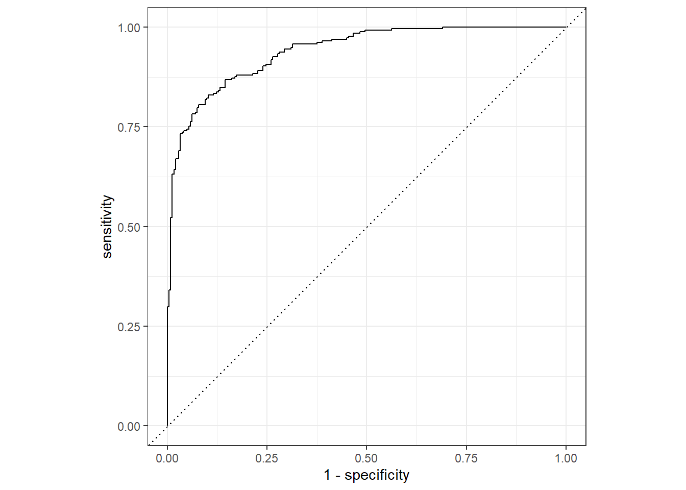

2.9.3 多分类变量-多分类模型

代码

data(hpc_cv)
tibble(hpc_cv) |>
  head()

# A tibble: 6 × 7
  obs   pred     VF      F       M          L Resample
  <fct> <fct> <dbl>  <dbl>   <dbl>      <dbl> <chr>   
1 VF    VF    0.914 0.0779 0.00848 0.0000199  Fold01  
2 VF    VF    0.938 0.0571 0.00482 0.0000101  Fold01  
3 VF    VF    0.947 0.0495 0.00316 0.00000500 Fold01  
4 VF    VF    0.929 0.0653 0.00579 0.0000156  Fold01  
5 VF    VF    0.942 0.0543 0.00381 0.00000729 Fold01  
6 VF    VF    0.951 0.0462 0.00272 0.00000384 Fold01

对于多分类模型，使用离散类预测的指标函数与二进制指标函数相同，如accuracy, mcc, f_meas等。

其他指标函数包括：

sensitivity：灵敏度，需要用estimator参数指定函数

代码

hpc_cv |>
  sensitivity(truth = obs, estimate = pred, estimator = "macro") # macro表示宏平均

# A tibble: 1 × 3
  .metric     .estimator .estimate
  <chr>       <chr>          <dbl>
1 sensitivity macro          0.560

代码

hpc_cv |>
  sensitivity(truth = obs, estimate = pred, estimator = "micro") # micro表示微平均

# A tibble: 1 × 3
  .metric     .estimator .estimate
  <chr>       <chr>          <dbl>
1 sensitivity micro          0.709

代码

hpc_cv |>
  sensitivity(truth = obs, estimate = pred, estimator = "macro_weighted") # macro_weighted表示加权宏平均

# A tibble: 1 × 3
  .metric     .estimator     .estimate
  <chr>       <chr>              <dbl>
1 sensitivity macro_weighted     0.709

roc_auc：多分类模型的AUC，必须向函数提供所有的类别概率列

代码

hpc_cv |>
  roc_auc(truth = obs, VF, F, M, L) # 这里也可以指定estimator参数

# A tibble: 1 × 3
  .metric .estimator .estimate
  <chr>   <chr>          <dbl>
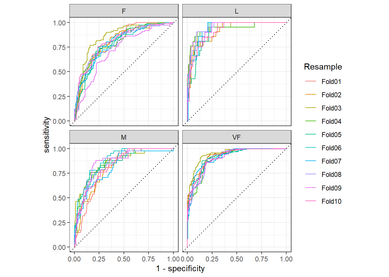
1 roc_auc hand_till      0.829

hpc_cv数据集中，有Resample列，是交叉验证的分组。可以利用group_by()函数为每个分组计算指标或作图，如图 2.8 所示。

代码

hpc_cv |>
  group_by(Resample) |>
  roc_curve(obs, VF, F, M, L) |>
  autoplot()

2.1 建模基础

2.2 练习数据和探索性数据分析

2.2.1 探索性数据分析-探索住宅特点

2.3 数据分割

2.3.1 简单随机抽样

2.3.2 分层抽样

2.3.3 交叉验证-验证集的分割

2.4 模型拟合-以线性回归为例

2.5 提取模型结果

2.6 模型预测

2.7 workflow

2.7.1 创建workflow对象

2.7.2 添加预处理器

2.7.3 添加变量

2.7.4 为workflow使用公式

2.7.4.1 基于树的模型

2.7.5 同时创建多个workflow

2.7.6 评估测试集

2.8 特征工程

2.8.1 创建特征工程

2.8.2 应用特征工程

2.8.3 其他特征工程示例

2.8.3.1 定性变量的处理

2.8.3.2 交互项的处理

2.8.3.3 样条函数

2.8.3.4 特征提取（PCA）

2.8.3.5 抽样技术

2.8.3.6 一般变换

2.8.3.7 自然语言处理

2.8.4 tidy

2.8.5 “roles”变量

2.9 模型性能评估

2.9.1 数值变量-回归模型

2.9.2 二分类变量-logistic回归模型

2.9.3 多分类变量-多分类模型

2.7.4 为`workflow`使用公式